The water cycle of a landscape

The water cycle of a landscape – A physical model

By Christian Lehr, Tobias Hohenbrink, Marcus Fahle, Marco Natkhin and Philipp Rauneker

The presented physical model shows the water cycle of a landscape. The model was jointly developed by PhD students and senior scientists of the Institute of Landscape Hydrology of the ZALF to illustrate hydrological issues. Using an aquarium enables to visualize the different ways of water flowing through a landscape in a limited space. In this way, important hydrological basics can be comprehended and understood. The model shows, how water behaves on and under the Earth’s surface. The landscape in the aquarium captures elements of landscapes that can be found in Northern Germany.

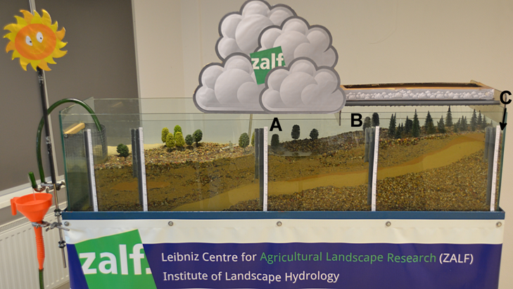
Figure 1 A model of the water cycle in a landscape.

The subsurface is made of different layers. These layers correspond to the geological layers of the North German Plain, as it developed during the Ice Ages. The uppermost layer is formed by a mix of sand and gravel. The lowest layer is made of gravel. In between there is a loam layer, which can be recognized by its light brown color. Gravel and sand are relatively coarse materials with large pores (in other words big spaces between the grains). In contrast, loam has much finer pores as also its grains are much finer and hardly visible.

The model landscape can be watered from above by an irrigation device. Behind the small clouds on the right hand side of the figure are pipes with small holes that are used to simulate rainfall. A part of the rain that falls on the surface reaches the pore space – it infiltrates. Water that concentrates in the subsurface and completely fills the pore space (so that there is no more air in the pores) is called groundwater.

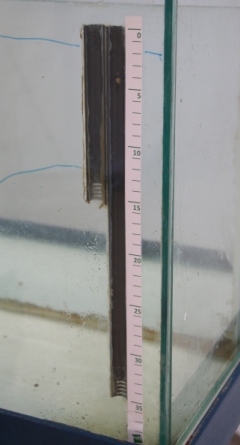
Figure 2 Construction of the gauges in the model.

On the front glass panel in figure 1 one can see gray pipes, which hydrologist term gauges. These pipes are open on the upper and the lower end. Figure 2 shows two gauges in detail. Groundwater can flow in and out. In the gauges the water level is always in equilibrium between the air pressure in the atmosphere and the water pressure of the groundwater at the lower end of the gauge. The lower ends of the gauges are installed at different depths to monitor different groundwater domains.

Water always tends to move on the path of the lowest resistance. Rivers, for example, flow along the ground surface from higher to lower altitudes until they end into a lake or eventually the sea.

Some soils are more permeable to water than others. The measure to describe these differences is the so-called hydraulic conductivity of the soil. The velocity of the subsurface water flow depends on the size of the pores and the prevailing pressure differences. The smaller the pores are and the smaller the pressure difference is the slower is the flow of the water through the soil layer. The pores of loam are so tiny that water in this layer hardly moves at all. Such layers are called aquitard. Water can flow easily through gravel and sand, according layers are termed aquifer. Anyhow, the velocities of the subsurface water flow are much lower than those at the surface, for instance the flow in a river.

On the left hand side of the model (see figure 1) is a free water surface, which in our example could represent the sea. The land surface declines from right to left in the direction to the sea. The sea in our model is therefore below the groundwater of the upper aquifer. Hence, this groundwater is flowing over the loam layers to the left into the sea.

In the middle of the landscape (in figure 1 under the right half of the big cloud) there is a lake with its catchment. The catchment of a water body is the region from which the water body receives water. A lake is simply a hollow mould in the landscape, where water can accumulate.

The lake is connected to the upper aquifer. Hence, its water level fluctuates with the groundwater level. For instance, when the groundwater level rises, water flows into the lake and the lake water level rises as well. The lake is recharged by groundwater. In case the lake water level keeps rising, the lake eventually spills and a river emerges. This river then flows to the sea.

A part of the water, which the highland receives as rain, passes through the lake on its way to the sea. In case of heavy rainfall, the water level in the river may rise higher than the river shores, causing a flood. On the other hand, water also infiltrates from the river into the groundwater, whenever the groundwater level is lower than the water level in the river. In dry areas or during times of drought it is even possible that all water from the river infiltrates and that the river runs dry.

Below the river on the left hand side of the model there is a lens of loam in the upper aquifer (the light brown spot on the left of figure 1). Contrary to a layer a lens is not continuous and only of small-scale. The lens of loam presents an obstacle to the water from the river that infiltrates above the lens. Thus, a subsurface “mountain of water” is formed and water flows from this mountain to both ends of the lens. On the right side of the lens water is even flowing against the main groundwater flow direction, which is in direction to the sea.

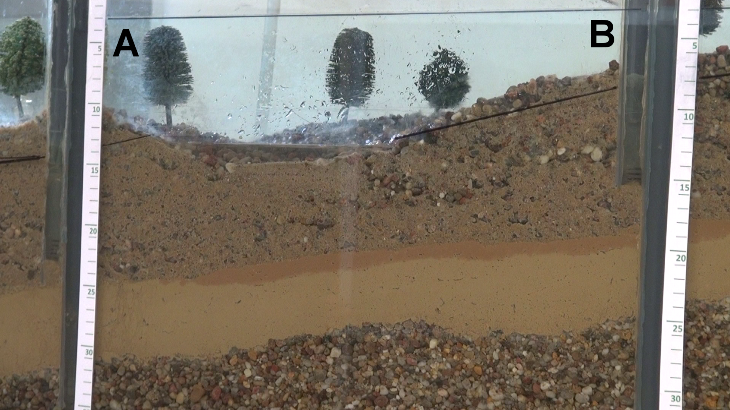
Figure 3 Pressure differences in both aquifers. Upper line: lower aquifer (confined conditions). Lower line: upper aquifer (unconfined conditions).

In the right gauges at positions A and B in figure 3 the water level is above the ground. How is that possible?

The gauges are arranged as pairs, from which the left gauge is connected to the upper aquifer, and the right one to the lower aquifer. The water of the lower aquifer cannot flow easily to the sea since the lower aquifer is covered by a loam layer. The loam layer works like a subsurface dam. At the right edge of the model (position C in figure 1), there is no loam layer and the rain (the water from the pipes) can directly infiltrate in the upper aquifer. In this case, water can easily infiltrate in the upper aquifer but the loam layer impedes the discharge of the water. Therefore, water gets stored in the aquifer and the groundwater level rises. If the rain does not stop, the lower aquifer would be eventually filled completely. Additional rain cannot infiltrate anymore but is discharged on the surface. In this case, the maximum groundwater level of the lower aquifer is reached. The groundwater level in the according gauge is equivalent to the ground surface of the right edge of the model. At this position, the aquifer is connected to the atmosphere.

In the gauge (= observation pipe) there is no loam or other material counteracting against the pressure from the groundwater. The groundwater pushes into the gauge and the water level in the gauge keeps rising until the groundwater pressure is in equilibrium with the atmospheric pressure. The atmospheric pressure is equal at all gauges.

The water pressure in the lower aquifer is nearly the same at all gauges. However, there are very small pressure differences as the conductivity of the loam layer is very low but not zero. These differences can hardly be seen and do not matter much for our following considerations. Therefore, the groundwater levels in all gauges connected to the lower aquifer can be assumed to be similar.

Hence, the groundwater level at the most right hand side gauge of figure 1 has the same height as in all the other gauges connected to the lower aquifer. In the model, the ground surface at position A is lower than at position C (figure 1). Since the maximum groundwater level of the lower aquifer is given by the ground surface at the right edge of the model, the groundwater level in the gauge at position A can exceed the ground surface by far.

Hydrologists call the aquifer in this situation a “confined aquifer”. A well installed under such conditions would not need any pump as the water would be pushed to the surface by the excess pressure in the aquifer. This kind of well is known as artesian well. In case the pressure of the aquifer is lowered, for instance by withdrawing water, also the groundwater level declines.

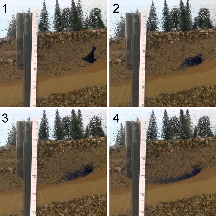
Ausbreitung eines (Farb-)Stoffes im Grundwasser

Figure 4 Propagation of a colorant in the groundwater during 4 times.

To the right of the gauge in figure 4 one can see a dark blue area in the upper aquifer, which is water that was coloured by ink. This technique is often used in hydrological experiments to visualize the water flow. Here, the coloured water moves towards the gauge over time. Imagine, the well would be used to extract drinking water and the ink would be a pollutant, then the drinking water would be contaminated. In this case, the source of contamination would not necessarily be close to the well. Contaminated water may travel a long way until reaching a drinking water well.

Unfortunately, in the real world we cannot directly look into the groundwater and see which way it is going. As we can see in the model, groundwater flows much slower than surface water. Therefore, the contamination of the drinking water well may have occurred long time ago.

For this reasons, hydrologists and water managers have to monitor groundwater constantly and need a lot of expertise. The knowledge about the behaviour of the water in the landscape has to be expended continuously and made accessible for the public. This is one of the most important tasks of our research institute.